Table of Contents
<texit info> author=Johnny Rieper, Bent Bisballe Nyeng and Kasper Sohn title=Marvin - The Balancing Robot. </texit>
Lab report 2 - PID Balance Control
Date: January 12nd 2009
Duration of activity: 8-12
Participants: Kasper, Bent and Johnny
Note that we returned to this subject several times during the following lab sessions.
Project Goal
Make the robot balance using mathematical modelling or simple PID parameter tuning.
Plan
- Discuss different control approaches and decide a course of action.
- Introduce the chosen controller
- Evaluate which features to use in the closed loop
- Make implementation of the chosen controller.
- Evaluate different methods of parameter tuning
Theory
Our Angle of Approach Towards Control Theory
Basically there are three approaches to our control problem, which we will describe briefly in an increasing order of complexity. The first method requires no more than an intuitive understanding of the tuning parameters in a given control loop as we consider the control plant as a black box. We simply implement a control loop by following the directions of the control loop as indicated in the following section Introducing the PID Controller. In this case we make no attempts to precalculate the stability issues e.g. using bode plots to observe phase margin as a function of our bandwidth. Instead we use a trial and error principle based on our intuitive understanding of the tuning parameters. The problem with this approach is that lack of knowledge about the dynamics of the control plant (the robot) if we do not succeed. We have no theoretical foundation.
The second approach is again to consider the control plant as a black box, but here we wish to estimate the characteristic transfer function of the plant. Recall that if we give an impulse to a filter we are given the filter characteristic by means of the impulse response. The analogy to control theory is to apply a step function and observe the transient response, which is illustrated on the figures in the following section Introducing the PID Controller. Depending on the order of the system we may need to apply a ramp or a parabola, but the principle is the same. By observing the rise time and settling time we may be able to estimate the transfer function and thereby to create a more solid foundation as to why the system is unstable and how large bandwidth we can obtain. This method is more complex since we need to be able to measure the transient response, which often requires expensive and precise equipment.
The third method is to derive a mathematical model of the dynamics of the control plant and this can be somewhat complex. In the case of a balancing robot it is helpful to look at the mathematical modelling of an inverted pendulum and there next to add the physical dimensions of the balancing robot. When working with modelling we end up with non linear equations, which is a problem as our controllers are linear. One common method is to use the state space representation and then to make a linearisation around the steady state point or the equilibrium. If our mathematical model is precise and close to the true physical model we obtain a great theoretical foundation for creating a stable system. This is exactly what Yorihisa Yamamoto1) has done and the result is outstanding. For this relatively short project however, the modelling is too comprehensive and we have seen several examples that the balancing can be achieved using the first method. We therefore rely on our intuitive understanding and use method one to implement our solution. We have decided to use the PID controller as we have already obtained some practical/intuitive understanding of the tuning parameters during LAB42).
Introducing the PID Controller
The digital implementation of a PID controller is actually based on very simple filtering techniques similar to what we described in the implementation section of LAB Session 1. Thus we need a digital filter integration and differentiation technique, which could be a trapezoidal method for integration and backward difference for the differentiation to give an example. The difference equations are used to present the numerical formula and the z-transform of those can then be used to evaluate transfer functions, which are useful to determine the frequency responses. We will not derive these expressions as they can be found in any decent control book. But be aware that we are in the digital domain where we often denote integration by 1/w instead of 1/s as in the continuous domain due to the z-transform, hence the transfer function and the control loop differs between the discrete and continuous domain. The PID control loop can be regarded simply as
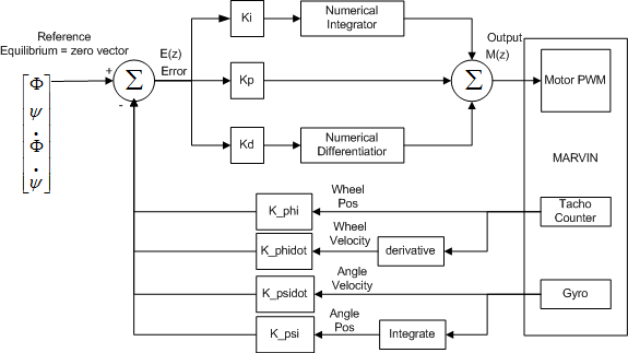
The plant is a term used in control theory to indicate the physical system, which is the robot. The Error signal is fed to the PWM control and the output is then subtracted from our reference values resulting an a new error signal. We see that the PID part of the loop is simply
<latex> \fracm_left_z_righte_left_z_right = D\left( w \right) = K_p + K_I \frac{1}{w} + K_D w </latex>
<latex> M\left( z \right) = \left( {K_p + K_I \frac{1}{w} + K_D w} \right)E\left( z \right) </latex>
<texit> \begin{equation} \fracm_left_z_righte_left_z_right = D\left( w \right) = K_p + K_I \frac{1}{w} + K_D w \end{equation} </texit>
<texit> \begin{equation} M\left( z \right) = \left( {K_p + K_I \frac{1}{w} + K_D w} \right)E\left( z \right) \end{equation} </texit>
This formulation is in the discrete frequency domain and we need to perform an inverse Z-transformation to go back to the discrete time domain. Instead of performing this explicitly we may just jump directly to the solution, since we already know what is required. We need a discrete time integration and differentiation and we can choose among several techniques. In the following we use the trapezoidal method and the backward difference as mentioned to obtain
<latex> m_rm_integral} \left[ {\left( {k + 1} \right)T} \right] = m\left( {kT} \right) + \frac{T}{2}\left\{ {e\left[ {\left( {k + 1} \right)T} \right] + e\left( {kT} \right)} \right\} </latex>
<latex> m_rm_derivative} \left[ {\left( {k + 1} \right)T} \right] = \frace_left_left_k_1_right_t_right_-_e_left_kt_right{T} </latex>
<latex> m\left[ {\left( {k + 1} \right)T} \right] = K_p e\left[ {\left( {k + 1} \right)T} \right] + K_I m_rm_integral} \left[ {\left( {k + 1} \right)T} \right] </latex> <latex> + K_D m_rm_derivative} \left[ {\left( {k + 1} \right)T} \right] </latex>
<texit> \begin{equation} m_rm_integral} \left[ {\left( {k + 1} \right)T} \right] = m\left( {kT} \right) + \frac{T}{2}\left\{ {e\left[ {\left( {k + 1} \right)T} \right] + e\left( {kT} \right)} \right\} \end{equation} </texit>
<texit> \begin{equation} m_rm_derivative} \left[ {\left( {k + 1} \right)T} \right] = \frace_left_left_k_1_right_t_right_-_e_left_kt_right{T} \end{equation} </texit>
<texit> \begin{equation} m\left[ {\left( {k + 1} \right)T} \right] = K_p e\left[ {\left( {k + 1} \right)T} \right] + K_I m_rm_integral} \left[ {\left( {k + 1} \right)T} \right] + K_D m_rm_derivative} \left[ {\left( {k + 1} \right)T} \right] \end{equation} </texit>
This is the output that is fed to the motor.
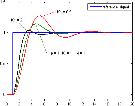
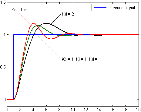
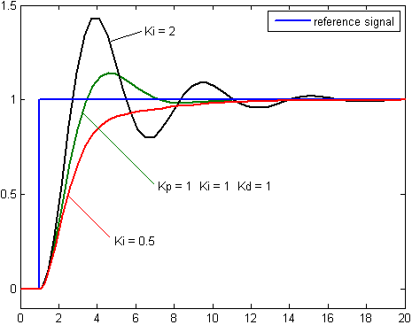
The above pictures are from 3)
By inspection we summarize the following. An increase in the proportional gain will create a larger overshoot, but reduce the steady state error and rise time. An increase in the integral controller also increase the overshoot, while eliminating the steady state error. If we increase the differential controller, we decrease the overshoot with no affect on the steady state error, but the bandwidth of the system will be reduced.
At wikipedia4) a pseudo code gives a nice interpretation of the numerical implementation, but note that the integration in this case is a running sum.
previous_error = 0
integral = 0
start:
  error = setpoint - actual_position
  integral = integral + error*dt
  derivative = (error - previous_error)/dt
  output = Kp*error + Ki*integral + Kd*derivative
  previous_error = error
  wait(dt)
  goto start
Further readings and inspiration are found at this homepage5), which was presented in week 3 of the course.
Defining the States in the Control Loop
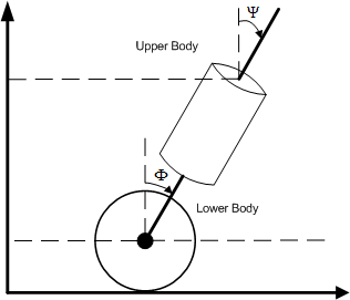
Now that we have established our choice of control loop, we must determine an error function. In a state space representation this corresponds to determining the states, which are defined through differential equations describing the dynamics of the control plant. Therefore we may turn to the model described in the documentation of Rich Chi Ooi6) , Yorihisa Yamamoto7) and several others and look for the terms included in the error function (the states). Not surprisingly, the states are identical in both these projects and naturally they have been chosen on basis of what others have done and what apparently is implemented in the commercially available Segway. They use four terms, which are the tilt angle,<latex>$\Psi$</latex><texit>$\Psi$</texit> , the angle velocity,<latex>$\dot{\Psi}$</latex><texit>${\dot{\Psi}}$</texit> , (its first derivative), the platform angular position, <latex>$\Phi$</latex><texit>$\Phi$</texit> , and the platform angular velocity,<latex>$\dot{\Phi}$</latex><texit>${\dot{\Phi}}$</texit> , (its first derivative).
This makes perfectly sense, since we need to drive the wheels in a direction that keeps the upper body of the robot in equilibrium. We therefore need sensor readings regarding the position of the wheels and the upper body in order to keep the wheels under the robot’s centre of gravity. It is easy to argument for the first order derivatives as well. From a mathematical point of view, the control point is a linearisation of second order non-linear equations (differential equations of the inverted pendulum) and therefore a descent approximation would include the first order terms to indicate the curvature as well. From a practical point of view, the curvature/velocity indicates how fast we are moving from the steady state point and these terms are very relevant in order for the error signal to rise relative to oscillations during balancing. We may also refer to this as feature extraction as we are selecting sufficient features to define the motion and position of this “inverted pendulum”. We sum up the states in the following diagram.
Parameters and Stability
The calculation of the right PID control parameters is essential to secure a stable system. This is called loop tuning. If loop tuning is not done according to the task at hand, the control system will become unstable i.e. the output will diverge. Oscillation might occur in this case. The only thing that will prevent divergence or oscillation is saturation or mechanical breakage. This may happen a lot when trying to produce a balancing robot and is generally not a problem due the great structural integrity, however if the controller is to control something else that might not be as rigid as our construction oscillation is always something to avoid in the first place.
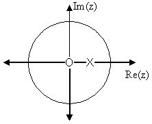
Loop tuning could be defined as adjusting the control loop parameters (Proportional gain(P), Integral gain (I) and Derivative gain(D)) to the optimum value for a desired control response. The z-transform for the controller should, in order to be stable obey the rules for a stable system, that is poles of the system should be located inside the unity circle, see diagram below.
Poles are represented with a cross and zeros with a circle. The shown diagram has no affiliation with our system. It is just provided as an example.
There are a number of different approaches when tuning PID parameters of which three will be described below. The methods that can be used range from no knowledge of the system to a full simulation of the system that can be used to calculate stability and set the exact parameters of the PID controller for optimum performance. One thing to note before talking about parameter tuning is the difference between online tuning and offline tuning. Online tuning means tuning when the system is running. That means one adjust parameters while the system is running. Offline tuning means take the control out of the plant, adjust the parameters and then re-engage the system. It is the later method we have used. The robot have been stopped, the parameters have en adjusted in the software, and lastly new firmware have been uploaded. Online tuning could have been used with a Bluetooth link between the robot and a PC from where new parameters could be uploaded on the fly.
Manual Tuning
This is a trial and error approach. You do not need to have any idea about the plant. The procedure is as follows:
- Set I and D values to zero
- Increase P until output of loop oscillates
- Set P to half the gain obtained in the previous step. P is now set for a quarter amplitude decay response type
- Increase I until steady state offset is correct. Too much will make the system unstable
- Increase D to get a faster settling time for the system.
These steps can be used in order to tune a system and it is preferable to do it to a system that is online.
The table below show the effects of increasing the parameters and can be used for fine tuning.
| Parameter | Rise Time | Overshoot | Settling Time | Steady State |
|---|---|---|---|---|
| P | Decrease | Increase | Small Change | Decrease |
| I | Decrease | Increase | Increase | Eliminate |
| D | Small Decrease | Decrease | Decrease | None |
Ziegler-Nichols Method
Another method developed makes use of what is called a critical gain. This is denoted <latex>K_{c}</latex><texit>$K_{c}$</texit> and is obtained in the same way as P is in the previous mentioned tuning method. Another parameter to be used is called <latex>P_{c}</latex><texit>$P_{c}$</texit> and denotes the oscillation period. The Ziegler-Nichols method can also be used if one only wants to make say a P or PI controller. The letters P, I and D in the vertical column denotes the type of controller whereas <latex>$K_p$</latex><texit>$K_p$</texit>, <latex>$K_i$</latex><texit>$K_i$</texit> and <latex>$K_d$</latex><texit>$K_d$</texit> denotes than for the parameters respectively.
| Control Type | <latex>$K_p$</latex><texit>$K_p$</texit> | <latex>$K_i$</latex><texit>$K_i$</texit> | <latex>$K_d$</latex><texit>$K_d$</texit> |
|---|---|---|---|
| P | <latex>0.5 K_{c}</latex><texit>$0.5 K_{c}$</texit> | - | - |
| I | <latex>0.45 K_{c}</latex><texit>$0.45 K_{c}$</texit> | <latex>\displaystyle\frac{1.2 K_{p}}{P_{c}}</latex><texit>$\displaystyle{1.2 K_{p}}/{P_{c}}$</texit> | - |
| D | <latex>0.6 K_{c}</latex><texit>$0.6 K_{c}$</texit> | <latex>\displaystyle{\frac{2 K_{p}}{P_{c}}}</latex><texit>$\displaystyle2_k_p/{P_{c}}}$</texit> | <latex>\displaystyle{\frac{K_{p} P_{c}}{8}}</latex><texit>$\displaystylek_p_p_c/{8}}$</texit> |
Tuning Software
There exist different kinds of tuning software. One of these could be 8). These software based solutions require a mathematical approach. In order to do this it is necessary to have a mathematical model of the plant to be controlled. The procedure induces an impulse into the system and then uses the controlled systems frequency response to design the PID parameters.
Summarize of Approaches
The three different approaches can be seen from the table below. In that table the advantages an disadvantages can me seen together with what knowledge is required.
| Method | Advantages | Disadvantage | Requirements |
|---|---|---|---|
| Manual Tuning | No math required (Online*) | Inaccurate | Some skill level |
| Ziegler-Nichols | Proven method (Online*) | Trial and error, pretty aggressive tuning | Ability to measure starting parameters such as <latex>$P_c$</latex><texit>$P_c$</texit> and <latex>$K_c$</latex><texit>$K_c$</texit> |
| Software Tools | Consistent tuning, Online or offline tuning, Allow for simulation beforehand | Expensive, knowledge about plant and development tools are required | Mathematical model |
* Online can in some cases be a disadvantage, e.g. a very long settling time. The time to try small adjustments may take days.
Implementation
First we present the software implementation, whereafter a short summary of the encountered problems is given.
Software - The Balance Control Class
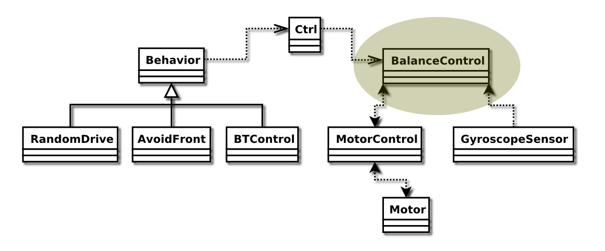 This class contains all the PID magic happening that makes Marvin keep its balance.
The balancing module reads the angles and the angle velocities from the gyroscope and motors, and uses these values (weighted) to feed to the PID control calculation which again produces the new power to apply to the motors.
These are the constants used as weights in PID control, and the error calculation:
| Symbol | Variable | Value |
|---|---|---|
| <latex>$K_p$</latex><texit>$K_p$</texit> | Kp | 1.0 |
| <latex>$K_i$</latex><texit>$K_i$</texit> | Ki | 0.2 |
| <latex>$K_d$</latex><texit>$K_d$</texit> | Kd | 0.2 |
| <latex>$K_\Psi$</latex><texit>$K_\Psi$</texit> | K_psi | 31.9978 |
| <latex>$K_\Phi$</latex><texit>$K_\Phi$</texit> | K_phi | 0.8703 |
| <latex>$K_\dot{\Psi}$</latex><texit>$K_{\dot{\Psi}}$</texit> | K_psidot | 0.6 |
| <latex>$K_\dot{\Phi}$</latex><texit>$K_{\dot{\Phi}}$</texit> | K_phidot | 0.02 |
<latex>$K_p$</latex><texit>$K_p$</texit>, <latex>$K_i$</latex><texit>$K_i$</texit> and <latex>$K_d$</latex><texit>$K_d$</texit> are the weights of the proportional, differential and
integral parts of the PID control. We name the gyroscope angle <latex>$\Psi$</latex><texit>$\Psi$</texit>,
and the Motor angle <latex>$\Phi$</latex><texit>$\Phi$</texit>, and their respective differentiates (angle
velocities) <latex>$\dot{\Psi}$</latex><texit>$\dot{\Psi}$</texit> and <latex>$\dot{\Phi}$</latex><texit>$\dot{\Phi}$</texit>, thus making <latex>$K_\Psi$</latex><texit>$K_\Psi$</texit> the weight of the <latex>$\Psi$</latex><texit>$\Psi$</texit> value in the error calculation, <latex>$K_\dot{\Psi}$</latex><texit>$K_{\dot{\Psi}}$</texit> then weight for the <latex>$\dot{\Psi}$</latex><texit>$\dot{\Psi}$</texit> and so on…
The sleep call at the end of the loop, reflects the max sample speed of the gyroscope, which should be is 300 times per second, 3.33msec between calls, but since the code itself takes up some time, the actual sleep value of 3msec seem to work appropriately.
The controls are added, in two places:
- To make Marvin move forward and backwards we add the tilt offset to the gyroscope angle (at the
gyro.getAngle()call).
- To make Marvin rotate wee add the left and right motor offsets directly to the right and left motor power (at the
motors.setPower(…)call).
The following is an excerpt from the BalanceControl class, showing the inner loop (which is running as a thread), that makes the error calculation, runs it through the PID, and finally adjusts the motor power accordingly.
public class BalanceControl extends Thread
{
  .
  .
  .

  public void run()

  {
    MotorControl motors = new MotorControl(Motor.C, Motor.B);
    GyroscopeSensor gyro = new GyroscopeSensor(SensorPort.S4);

    double int_error = 0.0;
    double prev_error = 0.0;

    while(true) {
      double Psi = gyro.getAngle() + ctrl.tiltAngle();
      double PsiDot = gyro.getAngleVelocity();

      double Phi = motors.getAngle();

      double PhiDot = motors.getAngleVelocity();

      double error = Psi * K_psi + Phi * K_phi + PsiDot * K_psidot + PhiDot * K_phidot;

      int_error += error; // Integral Error

      double deriv_error = error - prev_error; // Derivative Error
      prev_error = error;

      double pw = error * Kp + deriv_error * Kd + int_error * Ki;

      motors.setPower(pw + ctrl.leftMotorOffset(), pw + ctrl.rightMotorOffset());

      try { sleep(3); } catch(java.lang.InterruptedException e) { }
    }
  }
}
The full source code for this class can be found in the file BalanceControl.java in the Marvin code tarball 9)
Hardware Related Issues
At first we experienced severe stability problems as Marvin was highly sensitive to the offset of the gyroscope. The offset calibration did not appear to be stationary and this lead to diverging oscillations, which caused Marvin to crash over and over. (Fortunately the NXT module is quite solid.) We used great effort to find a solution to this problem and though the gyroscope tends to drift over time, we were able to find a stable combination of the tuning parameters causing Marvin to balance for several minutes - using only the tilt angle from the gyroscope and the PID control loop. At this point Marvin was balancing so we tried some preliminary attempts in order for Marvin to move forward/backward. This task was not as easy as expected and therefore the next lab report is devoted to the driving. It is important to notice, that at this point we did not use all the aforementioned states, since all four states contributed to an increasing set of gain combinations - it is not that easy to set all seven gains intuitively! We were only using the integration part of the gyroscope readings, but our suspicion at this point was closing in on the (lack of) states in the control loop. As we finally decided to work with all four states in the control loop, we found a strong combination of the four feedback gains. By adding these extra features we overcame the offset problems of the gyroscope to a satisfying degree. After some longer fine tuning of the parameters, Marvin showed a pretty stable behaviour and hereafter we were confident that he would be able to drive properly. It had to be a matter of finding the right approach, but this problem is addressed in the following lab report. The different attempts to resolve the gyroscope drifting is also adressed in the following lab report.


