Table of Contents
<texit info> author=Johnny Rieper, Bent Bisballe Nyeng and Kasper Sohn title=Marvin - The Balancing Robot. </texit>
Introduction
This project is the final part of the course Embedded Systems – Embodied Agents at the University of Aarhus 2008. The outline of the project is to demonstrate a practical implementation based on some of the theory acquired during preliminary lab sessions and lectures during the course. In our case we are building a balancing robot using the LEGO Mindstorm Kit and utilizing the LeJOS framework. The balancing robot was included in the preliminary lab sessions and we wish to make the robot able to think for itself and improve balancing when driving. Therefore we shall use the concept of behaviour models which is also a part of this course. This blog will serve as our “documentation” of the project and when necessary we will introduce a little background regarding sensors, actuators and controllers used in this project. The source code will be included in smaller segments following the development of the project, but the entire source code is available for download.
Our original project goal description can be found in its entirety in lab111)
Structure of this Document
This documents is divided into 7 parts. The introduction is the first part and is meant to give a general introduction the project, the LEGO Mindstorm NXT and the software structure as well as the naming conventions for easier reading.
Each lab report should not be read as a chronological evolution of the project, as there will be subjects mentioned that has not been fully implemented in that particular lab session. The lab reports are used to define different subjects of investigation.
The following 5 lap reports describes the process and the results.
- Lap report 1 describes how the robot was build and how the communication with the gyroscope is handled.
- Lap report 2 describes different control architectures, which one we use and how it is implemented to make the robot capable of balancing. Furthermore an introduction to tuning parameters and an evaluation of which features of an error signal to use is presented.
- Lap report 3 describes the steps involved in making the robot able to drive forward and backward and from there to be able to drive a predefined pattern. In this session we also present a supplementary section about DC servo motors based on the lectures.
- Lap report 4 describes the implementation of behaviour models which include behaviours such as the ability to drive autonomously and avoid obstacles.
- Lap report 5 describes how to make the robot remote controlled utilizing BlueTooth.
Finally there is a discussion/evaluation of the obtained results and a conclusion of the project as a whole.
Motivation
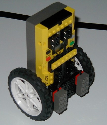
This problem of balancing an inverted pendulum is a nice delicate control problem and it has become the “Holy Grail” for many robot hobbyists around the world. The task of balancing a two wheeled robot may sound simple, but in reality many people have tried – and failed. In LAB42) we tried to make a self-balancing LEGO robot inspired by Steve Hassenplug's original Legway3) controlled by the RCX using light sensors – and failed. The task it not trivial as it requires knowledge and basic understanding of sensors, actuators and tuning parameters in the control loop. These challenges are appealing to us and we had many ideas of how to improve the implementation from LAB44). These ideas have laid the foundation of this final project, but we are not satisfied by making a simple balancing robot. In terms of the greater field of robotics, the balancing robot is almost purely mechanical, precluding the need for higher-level planning or behavioural programming that a more complex robot might require. Inputs over (discrete) time in the form of pendulum position readings are mapped algorithmically to output in the form of motor control. So we wanted to expand the project by adding behavioural programming using simple behaviours executed by a priority system. The motivation for behavioural programming was founded in LAB85), where we refer to some basic ideas of behaviour control. (for more advanced behaviour modelling look up Maja J Mataric) Another great motivation factor has been all the great videos from Youtube, where many people have tried to make a balancing robot using the LEGO Mindstorm kit. Most of them are very unstable and only capable of balancing, so it seems as a great challenge to make a remote controlled driving balancing robot with implemented behaviour models enabling the robot to interact with the environment. We were especially impressed and inspired by the outstanding implementation by Yorihisa Yamamoto6).
Literature Review
A great number of balancing robot projects exists on the internet and many papers on the subject have been published in IEEE journals. Furthermore commercial solutions are available e.g. the world famous Segway. The two wheel balancing robot has been researched by engineers, mathematicians, hobby robot enthusiasts and many more, therefore we shall comment very briefly on some of the papers and documents in which we found inspiration. Overall, the different projects are characterized by a very thorough analysis of both the dynamical model of the physical system and the appurtenant control theory. The time dedicated to this project does not allow us to choose a similar depth in terms of preliminary analysis and calculations, but we can certainly benefit from the experience and conclusions drawn in these pioneering projects. In the projects we have read, there is no preferred controller model, but there seems to be an agreement about which sensor features are needed in order to balance. This is quite promising for our project since we may settle with a simple controller if we manage to utilize proper sensors. (Of course, an advanced controller model would not be able to compensate for a bad choice of sensors). The control loop contains practically all elements that compose a control system, namely sensors, actuators, the plant and tuning parameters. All these factors are somewhat similar in the literature, but the numerical values must be set individually in every project.
In a paper by Rich Chi Ooi7) a two-wheeled differential driven mobile robot based on the inverted pendulum model is built as a platform to investigate the use of a Kalman filter for sensor fusion. The sensor fusion technique using a Kalman filter is a highly researched area and the idea is to combine different sensors in order to ensure higher stability in a given measurement. A common choice of sensor for a balancing robot is the gyro as it can measure the deviation from equilibrium. In practise however, the gyro tends to drift over time and thereby altering the reference value of the control system, hence making the entire system unstable. If we combine other sensors utilizing a Kalman filter we may be able to compensate for this drifting behaviour and keep the system in equilibrium. In the project an evaluation of the performance of a Linear Quadratic Regulator (LQR) and a Pole-placement controller is given as well. All calculations are presented analytically based on a derived dynamic model for a two wheeled inverted pendulum. Although the project illustrates some very exciting and relevant concepts, we have chosen to omit the use of sensor fusion since the Kalman Filter implementation would be beyond the scope of this project. Regarding the control loop we have no theoretical knowledge of the LQR control and again it would be unwise to focus on this type of control in our project. The pole placement controller is a possibility, but we considered this approach somewhat risky as this system will be unstable if the poles are placed too far on the left-hand plane. Therefore we decided to use a PID controller, which hopefully will prove to be adequate. In LAB48) we found quite promising results using light sensors and a PID controller.
Now let us turn towards the LEGO projects, which are numerous judging from the Youtube homepage. Two projects deserve special attention. Steven Hassenplug 9) has successfully constructed a balancing robot called Legway using the LEGO Mindstorms robotics kit. Two Electro-Optical Proximity Detector (EOPD) sensors is used to provide the tilt angle of the robot to the controller which is programmed in BrickOS, a C/C++ like programming language specifically for LEGO Mindstorms. This project was probably the first balancing robot using the Lego Mindstorm system and sparked many similar projects as this was an affordable platform for many hobbyists. A more recent project called NXTway-GS, written by Yorihisa Yamamoto10), is a self-balancing two-wheeled robot built with LEGO Mindstorms NXT and a Hitechnic gyroscope sensor. The final results of this project is very impressive and can be seen on youtube11) 12). Since this ultimately proves that a balancing system can be made using a gyroscope, we decided to use the exact same model by means of a building manual from the web page. The complete analytical solution by Yamamoto is somewhat complex, but this is mainly due to the simulation part of the project. With the physical model and sensors from this project, it should be possible to create our own balancing robot utilizing a simple PID controller.
Hardware
This section introduces the hardware used in this project. The sensors/actuators will be introduced further in the relevant lab sessions.
NXT Module
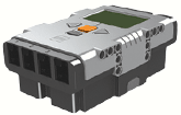
The NXT13) is the brain of a MINDSTORMS® robot.
Motor Ports
The NXT has three output ports for attaching motors - Ports A, B and C.
Sensor Ports
The NXT has four input ports for attaching sensors - Ports 1, 2, 3 and 4.
USB Port
Connect a USB cable to the USB port and download programs from the computer to the NXT (or upload data from the robot to the computer). It is also possible to use the wireless Bluetooth connection for uploading and downloading.
Technical Specifications
- 32-bit ARM7 microcontroller
- 256 Kbytes FLASH, 64 Kbytes RAM
- 8-bit AVR microcontroller
- 4 Kbytes FLASH, 512 Byte RAM
- Bluetooth wireless communication (Bluetooth Class II V2.0 compliant)
- USB full speed port (12 Mbit/s)
- 4 input ports, 6-wire cable digital platform (One port includes a IEC 61158 Type 4/EN 50 170 compliant expansion port for future use)
- 3 output ports, 6-wire cable digital platform
- 100 x 64 pixel LCD graphical display
- Loudspeaker - 8 kHz sound quality. Sound channel with 8-bit resolution and 2-16 kHz sample rate.
- Power source: 6 AA batteries
The Gyroscope
Measure the additional dimension of rotation with the NXT Gyro Sensor. This sensor that lets you accurately detect rotation for your NXT projects. The NXT Gyro Sensor returns the number of degrees per second of rotation as well as indicating the direction of rotation. Measure +/- 360° per second and build robots that can balance, swing or perform other functions where measurement of rotation is essential.
The Ultrasonic Sensor
The Ultrasonic Sensor enables your robot to see and detect objects. You can also use it to make your robot avoid obstacles, sense and measure distance, and detect movement.The Ultrasonic Sensor measures distance in centimeters and in inches. It is able to measure distances from 0 to 255 centimeters with a precision of +/- 3 cm.
The DC Servo Motor
There are three Servo Motors included in the Mindstorm kit. Each motor has a built-in Rotation Sensor. This lets your control your robot’s movements precisely. The Rotation Sensor measures motor rotations in degrees or full rotations (accuracy of +/- one degree). One rotation is equal to 360 degrees, so if you set a motor to turn 180 degrees, its output shaft will make half a turn. The built-in Rotation Sensor in each motor also lets you set different speeds for your motors (by setting different power parameters in the software). The motors have sufficient power in order to make the robot balance.
Software
The code is purely written in the Java syntax through the LeJOS NXT framework14).
We use CamelCase notation15) for both the methods and variable names.
All classes are fully documented by the javadoc documentation conventions16).
Class Overview
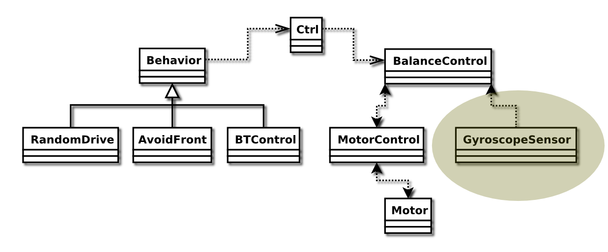
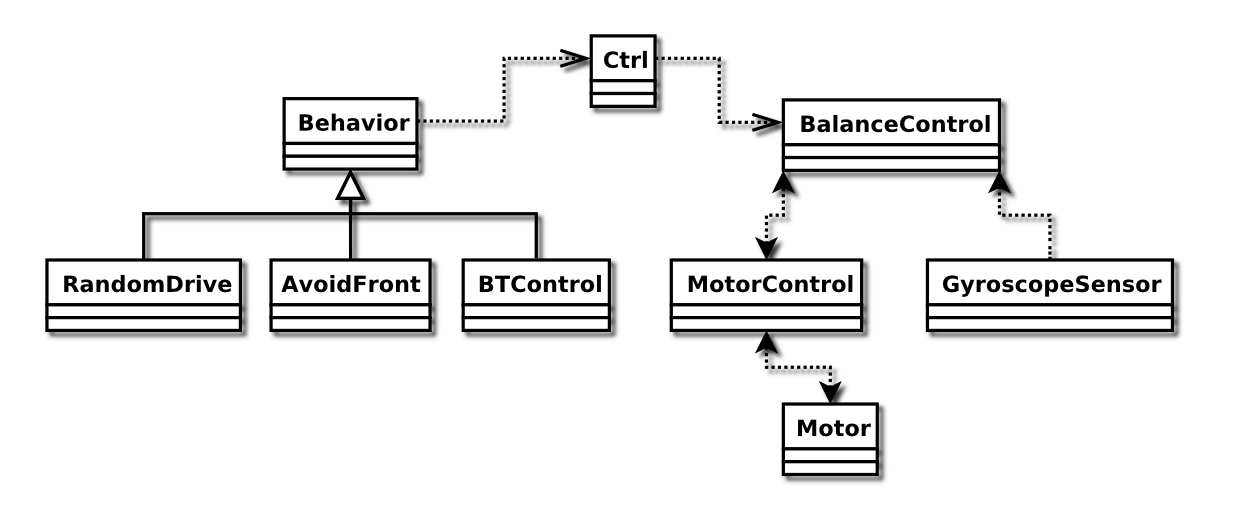 The above figure illustrates all the important classes in the project as well as their relations to each other.
A tarball with the source code can be fetched here: marvin-1.0.tar.gz
Apart from the classes shown in the class overview, there are the Print class, which has been used for debugging purposes (writes number to the display, with a label, and possibility to write doubles), the PCController, which communicate with the BTController class, and finally the Marvin class which contains the main, that simply instantiates all the objects and activates all the threads. these classes can also be seen in the source code tarball.
Take note that printing out to the LCD is a very expensive task, and since the art of balancing is very sensitive, the print class cannot be used while actually running.
The Name
The name “Marvin” has been taken from “The Hitchhikers Guide to the Galaxy” in which an android bears that exact name. He is also called “Marvin, the paranoid android”17), which refers to his sad mood, caused by a severe depression, and boredom, a behaviour we saw mirrored in the way our particular robot was moving and behaving.
Lab Report 1 - Gyroscope Communication
Date: January 2nd 2009
Duration of activity: 8-14
Participants: Kasper, Bent and Johnny
Goal
Make Marvin able to communicate with gyroscope.
Plan
- Build the robot in LEGO following the instructions on the mathworks website18).
- Make a test program to test if the gyroscope is working.
- Find or create a class for the gyroscope communication.
Theory
Analogue to Digital Conversion and Limitations
The main problem when dealing with sensors is that the real world is continuous and when we want to interpret these data it has to be digitized (discretized) in some way. This is done with an analogue to digital converter (A/D-converter or simply ADC). The opposite applies when we have a digital value, such as an integer and this is converted to an analogue value (D/A-converter or DAC). This in itself is a huge area, and the conversion itself will not be covered further. The important thing to remember is that in order to get an appropriate estimate of the real world the samples that you take from your sensor has to be taken often enough so that you will not loose vital data. How often one should sample depends on the application, but as a rule of thumb one should sample minimum twice as fast as the highest rate of different that will occur. As an example, if you want to reproduce a sinus with the frequency of 100 Hz, you will have to sample with 200 Hz. A higher sample rate will produce a more accurate output, but will also need more computational power. The gyroscope utilizes the ADC so that it is possible to get readings from the gyroscope.
Gyroscope
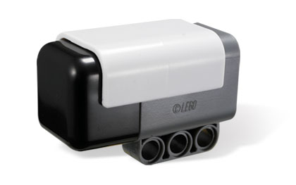
The gyroscope used has been purchased from HiTechnic 19) and is shown on the picture below. The housing is a standard Lego Mindstorm sensor so it fits with other sensors, and is more easily incorporated in a building scheme which purely uses LEGO bricks.
The gyroscope is produced to work seamless with the LEGO NXT Brick. It connects to the NXT using a standard wire and utilizes the analogue interface. The gyroscope contains a single axis gyroscopic sensor that detects rotation and returns a value representing the number of degrees per second of rotation. The gyroscope sensor measures up to +/- 360 degrees per second of rotation and these readings will be signed if the correct offset is used.
As not all gyroscopes are identical there will be some minor differences in the offset, but the manual that came along with the gyroscope, indicates this to be around 620. This is the offset value has to be subtracted from the readings from the gyroscope in order to get a signed reading.
The sensor can be read 300 times per second (an interval of 3.33 times per second), which correspond to a sample rate of 300 Hz.
The gyroscope operates in relative values, which means that it can not tell where e.g. upright is. One have to “show” where that is, and from there the gyroscope readings will show how fast the gyroscope is moving from that position. To get an accurate reading it might be necessary to read the value from the right position over some time (e.g. 2 seconds) and from that generate a mean value. This mean value of offset can then be used in further calculations to increase accuracy.
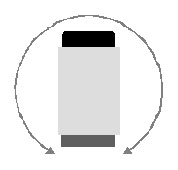
The axis of measurement is in the vertical plane with the gyroscope sensor positioned with the black end cap facing upwards, as illustrated in thye figure below.
The correct placement of the gyroscope can be seen in the building instructions
Building the Robot
Preliminary considerations
Our primary goal is to make a balancing robot, and therefore it would be nice to eliminate the possibility of failure due to a bad build. This is the reason why we chose to re-use the instructions provided as seen in the building manual20). We know that this design is working. Another reason for choosing this design is that there exists extensive simulation material on this specific robot, which might make it easier to fine-tune the parameters later on.
The Build
The build is pretty straight forward, as the building instructions is well written and also accompanied by photos. One thing to note though, is that the robot is fairly symmetric, so building instructions is only provided for one side of the robot and it is up to the builder to mirror the other side. This is however no problem because of the good photos.
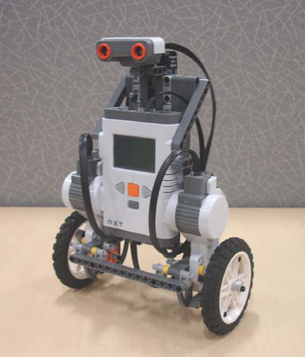
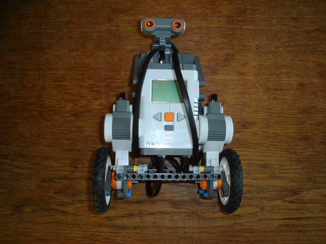
The finished robot can be seen in the picture below.
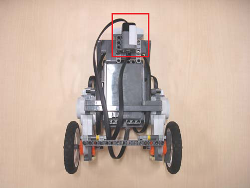
One thing worth noting is that the ultrasonic sensor is shifted slightly to the left. This is because it is important that the gyroscopes fix point is centered on the vertical axis of the robot. Positioning of the gyroscope is well documented in the building instructions. Below is a photo of the gyroscope in place.
Peripheral Connections
| Sensor | Output | Unit | Data Type | Maximum Sample [1/sec] | Port |
|---|---|---|---|---|---|
| Rotary Encoder Left * | angle | deg | int32 | 1000 | B |
| Rotary Encoder Right * | angle | deg | int32 | 1000 | C |
| Ultrasonic Sensor | distance | cm | int32 | 50 (N1) | 2 |
| Gyroscope Sensor | angular speed | deg/sec | uint16 | 300 | 4 |
| Actuator | Input | Unit | Data Type | Maximum Sample [1/sec] | Port |
|---|---|---|---|---|---|
| DC Motor Left * | PWM | % | int8 | 500 | B |
| DC Motor Right * | PWM | % | int8 | 500 | C |
*The rotary encoders and DC Motors (left and right respectively) utilizes the same port.
Pros and Cons About the Design
As mentioned earlier, this is a well documented and working design. This is of great importance, because we can eliminate this as a factor of error later on. Another issue that have proven important in our experiments is the ability to easily remove the battery for recharging. This may not seem important at this point, but the characteristics of the voltage applied to the motors vary greatly with the charge level of the battery, and therefore the behaviour of the motors varies. It is therefore a nice feature that the battery is easy to remove without tearing the robot apart.
In the group we discussed what effect the wheel diameter will have on the robot. Wheels with a larger diameter will travel a longer than smaller wheels for the same amount of power applied to the motor on which the wheel is mounted. We decided that the resolution of the wheel rotational properties were accurate enough to go with the larger wheels, and these wheels were also used in the design we used in the first place, and therefore was a well-proven design.
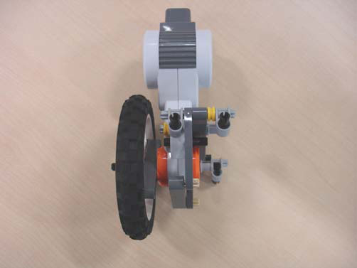
A thing worth mentioning is the construction of the wheel mounting point and wheelbase which can be seen on the picture below
This construction provides a rigid frame that will prevent structural wobbling. This is important because of the sudden movements forward and backward motions a balancing robot evidently will make.
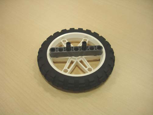
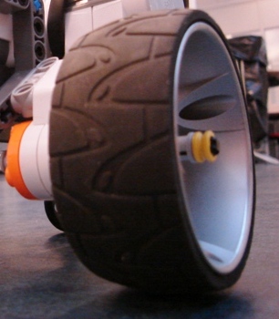
The wheel mounting point is cleverly made so that there will be no loss of power between the motor and the wheel. We used the standard wheels throughout testing, but found these to have to much friction when driven on rugged carpet. Although they have a cleverly designed mounting point we found that this was not necessary in our implementation and opted to go with the wheels shown below.
Implementation
Numerical Readings from the Gyroscope
A gyroscope measures degrees per second or simply angle velocity and therefore we must use numerical integration in order to get the angle. A gyroscope has a bias which is simply an offset and naturally we want to eliminate this offset by calibration methods at the beginning of the program. If we do not calibrate, the integration, e.g. a running sum, will add the offset contribution for every sample and diverge resulting in an unstable system. If we calibrate the integral, this problem will be reduced, but unfortunately the bias of the gyroscope tends to drift and therefore one needs to recalibrate if possible or find other heuristic methods in order to avoid an escalation of the error. Sensor fusion is suggested, which rely on the somewhat complex implementation of the Kalman filter, which may combine sensor inputs an re-estimate the most likely bias value while offering an indication of how much trust we may put in this value. A sensor fusion could be used to combine an accelerometer or inclinometer with the gyroscope, but it seems a bit ambitious to implement a Kalman solution given the scope of this project - also keeping in mind that there are many other areas of improvement that should be evaluated first.
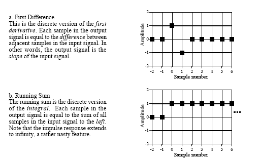
In order to do a discrete integration we simply need to look at a simple recursive difference equation, which in this case will be a running sum. Recall the difference equations for simple first order derivatives and a very simple integration:
Integration: <latex>y_n=x_n+y_{n-1}</latex><texit>$y_n=x_n+y_{n-1}$</texit>
First difference: <latex>y_n=x_n+x_{n-1}</latex><texit>$y_n=x_n+x_{n-1}$</texit>
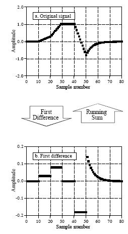
Each sample in the output signal is a sum of weighted samples from the input. The reason for pointing out the first order derivative as well is that they (of course) are closely related which becomes clear in the illustration below. 21)
There are many types of algorithms for numerical integrations that are far more advanced and all of them or based on some kind of interpolation technique, but for now we will rely on the simplest form which is the running sum.
Programming
LeJOS has its own GyroSensor class22). But apparently it only supports reading of the raw gyroscope values, and offers no interpretations (it is essentially just a wrapper of the SensorPort class, with an offset). We therefore programmed our own GyroscopeSensor class, with methods for reading out both the angle velocity, and the calculated (integrated angle velocity over time) angle.
This class wraps the gyroscope sensor, and offers readouts as either angle velocities, or as integrated angle velocities over time (angles).
The angle velocities can be read raw from the sensor port, but must be subtracted with an offset defining the stand-still gyroscope. This value is according to the documentation approximately 620, but may vary from gyroscope to gyroscope. We made some experiments and found the value 595.5 to be pretty accurate.
This value is however not accurate enough when run over a large quantity of time, which will make the integration drift, thereby making Marvin unable to keep its balance.
The solution was to use the measured value as an initial value, and then use a weighted average of all measured angles over time, where the last measured angle is weighted very low. We tested the solution with a variety of values, and found the value 0.999999 to be pretty good (one might think the having a static 595.5 might do the same, but experiments show otherwise).
These constants are hard coded into the program with the following names and values:
| Variable | Value |
|---|---|
| lastOffset | 595.5 |
| a | 0.999999 |
For the integration over time algorithm we use a simple sum multiplied by the delta time since last call. This delta time is acquired by calling the System.currentTimeMillis() method, which reports the number of milliseconds since the NXT was been turned on.
In the following excerpt from the GyroscopeSensor class can be seen the weighted average algorithm in the getAngleVelocity() method, and the integration over time algorithm in then getAngle() method.
public class GyroscopeSensor
{
  private SensorPort port;

  .
  .
  .

  private double getAngleOffset()
  {
    double offset = lastOffset * a + (1.0 - a) * (double)port.readValue();
    lastOffset = offset;
    return offset;
  }


  .
  .
  .

  public double getAngle()
  {
    int now = (int)System.currentTimeMillis();
    int delta_t = now - lastGetAngleTime;

    // Make sure we only add to the sum when there has actually
    // been a previous call (delta_t == now if its the first call).
    if(delta_t != now) {
      angle += getAngleVelocity() * ((double)delta_t / 1000.0);
    }

    lastGetAngleTime = now;

    return angle;
  }
}
The full source code for this class can be found in the file GyroscopeSensor.java in the Marvin code tarball 23)
Lab report 2 - PID Balance Control
Date: January 12nd 2009
Duration of activity: 8-12
Participants: Kasper, Bent and Johnny
Note that we returned to this subject several times during the following lab sessions.
Project Goal
Make the robot balance using mathematical modelling or simple PID parameter tuning.
Plan
- Discuss different control approaches and decide a course of action.
- Introduce the chosen controller
- Evaluate which features to use in the closed loop
- Make implementation of the chosen controller.
- Evaluate different methods of parameter tuning
Theory
Our Angle of Approach Towards Control Theory
Basically there are three approaches to our control problem, which we will describe briefly in an increasing order of complexity. The first method requires no more than an intuitive understanding of the tuning parameters in a given control loop as we consider the control plant as a black box. We simply implement a control loop by following the directions of the control loop as indicated in the following section Introducing the PID Controller. In this case we make no attempts to precalculate the stability issues e.g. using bode plots to observe phase margin as a function of our bandwidth. Instead we use a trial and error principle based on our intuitive understanding of the tuning parameters. The problem with this approach is that lack of knowledge about the dynamics of the control plant (the robot) if we do not succeed. We have no theoretical foundation.
The second approach is again to consider the control plant as a black box, but here we wish to estimate the characteristic transfer function of the plant. Recall that if we give an impulse to a filter we are given the filter characteristic by means of the impulse response. The analogy to control theory is to apply a step function and observe the transient response, which is illustrated on the figures in the following section Introducing the PID Controller. Depending on the order of the system we may need to apply a ramp or a parabola, but the principle is the same. By observing the rise time and settling time we may be able to estimate the transfer function and thereby to create a more solid foundation as to why the system is unstable and how large bandwidth we can obtain. This method is more complex since we need to be able to measure the transient response, which often requires expensive and precise equipment.
The third method is to derive a mathematical model of the dynamics of the control plant and this can be somewhat complex. In the case of a balancing robot it is helpful to look at the mathematical modelling of an inverted pendulum and there next to add the physical dimensions of the balancing robot. When working with modelling we end up with non linear equations, which is a problem as our controllers are linear. One common method is to use the state space representation and then to make a linearisation around the steady state point or the equilibrium. If our mathematical model is precise and close to the true physical model we obtain a great theoretical foundation for creating a stable system. This is exactly what Yorihisa Yamamoto24) has done and the result is outstanding. For this relatively short project however, the modelling is too comprehensive and we have seen several examples that the balancing can be achieved using the first method. We therefore rely on our intuitive understanding and use method one to implement our solution. We have decided to use the PID controller as we have already obtained some practical/intuitive understanding of the tuning parameters during LAB425).
Introducing the PID Controller
The digital implementation of a PID controller is actually based on very simple filtering techniques similar to what we described in the implementation section of LAB Session 1. Thus we need a digital filter integration and differentiation technique, which could be a trapezoidal method for integration and backward difference for the differentiation to give an example. The difference equations are used to present the numerical formula and the z-transform of those can then be used to evaluate transfer functions, which are useful to determine the frequency responses. We will not derive these expressions as they can be found in any decent control book. But be aware that we are in the digital domain where we often denote integration by 1/w instead of 1/s as in the continuous domain due to the z-transform, hence the transfer function and the control loop differs between the discrete and continuous domain. The PID control loop can be regarded simply as
The plant is a term used in control theory to indicate the physical system, which is the robot. The Error signal is fed to the PWM control and the output is then subtracted from our reference values resulting an a new error signal. We see that the PID part of the loop is simply
<latex> \fracm_left_z_righte_left_z_right = D\left( w \right) = K_p + K_I \frac{1}{w} + K_D w </latex>
<latex> M\left( z \right) = \left( {K_p + K_I \frac{1}{w} + K_D w} \right)E\left( z \right) </latex>
<texit> \begin{equation} \fracm_left_z_righte_left_z_right = D\left( w \right) = K_p + K_I \frac{1}{w} + K_D w \end{equation} </texit>
<texit> \begin{equation} M\left( z \right) = \left( {K_p + K_I \frac{1}{w} + K_D w} \right)E\left( z \right) \end{equation} </texit>
This formulation is in the discrete frequency domain and we need to perform an inverse Z-transformation to go back to the discrete time domain. Instead of performing this explicitly we may just jump directly to the solution, since we already know what is required. We need a discrete time integration and differentiation and we can choose among several techniques. In the following we use the trapezoidal method and the backward difference as mentioned to obtain
<latex> m_rm_integral} \left[ {\left( {k + 1} \right)T} \right] = m\left( {kT} \right) + \frac{T}{2}\left\{ {e\left[ {\left( {k + 1} \right)T} \right] + e\left( {kT} \right)} \right\} </latex>
<latex> m_rm_derivative} \left[ {\left( {k + 1} \right)T} \right] = \frace_left_left_k_1_right_t_right_-_e_left_kt_right{T} </latex>
<latex> m\left[ {\left( {k + 1} \right)T} \right] = K_p e\left[ {\left( {k + 1} \right)T} \right] + K_I m_rm_integral} \left[ {\left( {k + 1} \right)T} \right] </latex> <latex> + K_D m_rm_derivative} \left[ {\left( {k + 1} \right)T} \right] </latex>
<texit> \begin{equation} m_rm_integral} \left[ {\left( {k + 1} \right)T} \right] = m\left( {kT} \right) + \frac{T}{2}\left\{ {e\left[ {\left( {k + 1} \right)T} \right] + e\left( {kT} \right)} \right\} \end{equation} </texit>
<texit> \begin{equation} m_rm_derivative} \left[ {\left( {k + 1} \right)T} \right] = \frace_left_left_k_1_right_t_right_-_e_left_kt_right{T} \end{equation} </texit>
<texit> \begin{equation} m\left[ {\left( {k + 1} \right)T} \right] = K_p e\left[ {\left( {k + 1} \right)T} \right] + K_I m_rm_integral} \left[ {\left( {k + 1} \right)T} \right] + K_D m_rm_derivative} \left[ {\left( {k + 1} \right)T} \right] \end{equation} </texit>
This is the output that is fed to the motor.
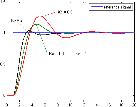
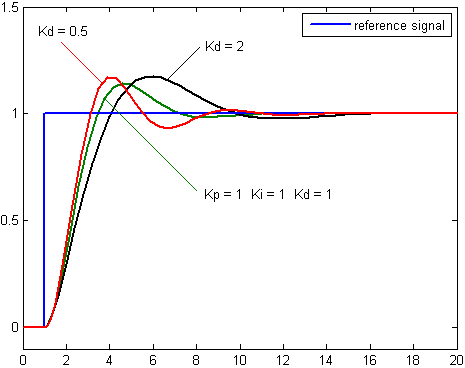
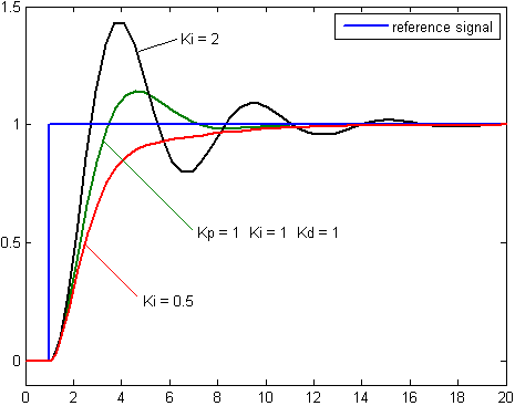
The above pictures are from 26)
By inspection we summarize the following. An increase in the proportional gain will create a larger overshoot, but reduce the steady state error and rise time. An increase in the integral controller also increase the overshoot, while eliminating the steady state error. If we increase the differential controller, we decrease the overshoot with no affect on the steady state error, but the bandwidth of the system will be reduced.
At wikipedia27) a pseudo code gives a nice interpretation of the numerical implementation, but note that the integration in this case is a running sum.
previous_error = 0
integral = 0
start:
  error = setpoint - actual_position
  integral = integral + error*dt
  derivative = (error - previous_error)/dt
  output = Kp*error + Ki*integral + Kd*derivative
  previous_error = error
  wait(dt)
  goto start
Further readings and inspiration are found at this homepage28), which was presented in week 3 of the course.
Defining the States in the Control Loop
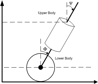
Now that we have established our choice of control loop, we must determine an error function. In a state space representation this corresponds to determining the states, which are defined through differential equations describing the dynamics of the control plant. Therefore we may turn to the model described in the documentation of Rich Chi Ooi29) , Yorihisa Yamamoto30) and several others and look for the terms included in the error function (the states). Not surprisingly, the states are identical in both these projects and naturally they have been chosen on basis of what others have done and what apparently is implemented in the commercially available Segway. They use four terms, which are the tilt angle,<latex>$\Psi$</latex><texit>$\Psi$</texit> , the angle velocity,<latex>$\dot{\Psi}$</latex><texit>${\dot{\Psi}}$</texit> , (its first derivative), the platform angular position, <latex>$\Phi$</latex><texit>$\Phi$</texit> , and the platform angular velocity,<latex>$\dot{\Phi}$</latex><texit>${\dot{\Phi}}$</texit> , (its first derivative).
This makes perfectly sense, since we need to drive the wheels in a direction that keeps the upper body of the robot in equilibrium. We therefore need sensor readings regarding the position of the wheels and the upper body in order to keep the wheels under the robot’s centre of gravity. It is easy to argument for the first order derivatives as well. From a mathematical point of view, the control point is a linearisation of second order non-linear equations (differential equations of the inverted pendulum) and therefore a descent approximation would include the first order terms to indicate the curvature as well. From a practical point of view, the curvature/velocity indicates how fast we are moving from the steady state point and these terms are very relevant in order for the error signal to rise relative to oscillations during balancing. We may also refer to this as feature extraction as we are selecting sufficient features to define the motion and position of this “inverted pendulum”. We sum up the states in the following diagram.
Parameters and Stability
The calculation of the right PID control parameters is essential to secure a stable system. This is called loop tuning. If loop tuning is not done according to the task at hand, the control system will become unstable i.e. the output will diverge. Oscillation might occur in this case. The only thing that will prevent divergence or oscillation is saturation or mechanical breakage. This may happen a lot when trying to produce a balancing robot and is generally not a problem due the great structural integrity, however if the controller is to control something else that might not be as rigid as our construction oscillation is always something to avoid in the first place.
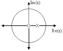
Loop tuning could be defined as adjusting the control loop parameters (Proportional gain(P), Integral gain (I) and Derivative gain(D)) to the optimum value for a desired control response. The z-transform for the controller should, in order to be stable obey the rules for a stable system, that is poles of the system should be located inside the unity circle, see diagram below.
Poles are represented with a cross and zeros with a circle. The shown diagram has no affiliation with our system. It is just provided as an example.
There are a number of different approaches when tuning PID parameters of which three will be described below. The methods that can be used range from no knowledge of the system to a full simulation of the system that can be used to calculate stability and set the exact parameters of the PID controller for optimum performance. One thing to note before talking about parameter tuning is the difference between online tuning and offline tuning. Online tuning means tuning when the system is running. That means one adjust parameters while the system is running. Offline tuning means take the control out of the plant, adjust the parameters and then re-engage the system. It is the later method we have used. The robot have been stopped, the parameters have en adjusted in the software, and lastly new firmware have been uploaded. Online tuning could have been used with a Bluetooth link between the robot and a PC from where new parameters could be uploaded on the fly.
Manual Tuning
This is a trial and error approach. You do not need to have any idea about the plant. The procedure is as follows:
- Set I and D values to zero
- Increase P until output of loop oscillates
- Set P to half the gain obtained in the previous step. P is now set for a quarter amplitude decay response type
- Increase I until steady state offset is correct. Too much will make the system unstable
- Increase D to get a faster settling time for the system.
These steps can be used in order to tune a system and it is preferable to do it to a system that is online.
The table below show the effects of increasing the parameters and can be used for fine tuning.
| Parameter | Rise Time | Overshoot | Settling Time | Steady State |
|---|---|---|---|---|
| P | Decrease | Increase | Small Change | Decrease |
| I | Decrease | Increase | Increase | Eliminate |
| D | Small Decrease | Decrease | Decrease | None |
Ziegler-Nichols Method
Another method developed makes use of what is called a critical gain. This is denoted <latex>K_{c}</latex><texit>$K_{c}$</texit> and is obtained in the same way as P is in the previous mentioned tuning method. Another parameter to be used is called <latex>P_{c}</latex><texit>$P_{c}$</texit> and denotes the oscillation period. The Ziegler-Nichols method can also be used if one only wants to make say a P or PI controller. The letters P, I and D in the vertical column denotes the type of controller whereas <latex>$K_p$</latex><texit>$K_p$</texit>, <latex>$K_i$</latex><texit>$K_i$</texit> and <latex>$K_d$</latex><texit>$K_d$</texit> denotes than for the parameters respectively.
| Control Type | <latex>$K_p$</latex><texit>$K_p$</texit> | <latex>$K_i$</latex><texit>$K_i$</texit> | <latex>$K_d$</latex><texit>$K_d$</texit> |
|---|---|---|---|
| P | <latex>0.5 K_{c}</latex><texit>$0.5 K_{c}$</texit> | - | - |
| I | <latex>0.45 K_{c}</latex><texit>$0.45 K_{c}$</texit> | <latex>\displaystyle\frac{1.2 K_{p}}{P_{c}}</latex><texit>$\displaystyle{1.2 K_{p}}/{P_{c}}$</texit> | - |
| D | <latex>0.6 K_{c}</latex><texit>$0.6 K_{c}$</texit> | <latex>\displaystyle{\frac{2 K_{p}}{P_{c}}}</latex><texit>$\displaystyle2_k_p/{P_{c}}}$</texit> | <latex>\displaystyle{\frac{K_{p} P_{c}}{8}}</latex><texit>$\displaystylek_p_p_c/{8}}$</texit> |
Tuning Software
There exist different kinds of tuning software. One of these could be 31). These software based solutions require a mathematical approach. In order to do this it is necessary to have a mathematical model of the plant to be controlled. The procedure induces an impulse into the system and then uses the controlled systems frequency response to design the PID parameters.
Summarize of Approaches
The three different approaches can be seen from the table below. In that table the advantages an disadvantages can me seen together with what knowledge is required.
| Method | Advantages | Disadvantage | Requirements |
|---|---|---|---|
| Manual Tuning | No math required (Online*) | Inaccurate | Some skill level |
| Ziegler-Nichols | Proven method (Online*) | Trial and error, pretty aggressive tuning | Ability to measure starting parameters such as <latex>$P_c$</latex><texit>$P_c$</texit> and <latex>$K_c$</latex><texit>$K_c$</texit> |
| Software Tools | Consistent tuning, Online or offline tuning, Allow for simulation beforehand | Expensive, knowledge about plant and development tools are required | Mathematical model |
* Online can in some cases be a disadvantage, e.g. a very long settling time. The time to try small adjustments may take days.
Implementation
First we present the software implementation, whereafter a short summary of the encountered problems is given.
Software - The Balance Control Class
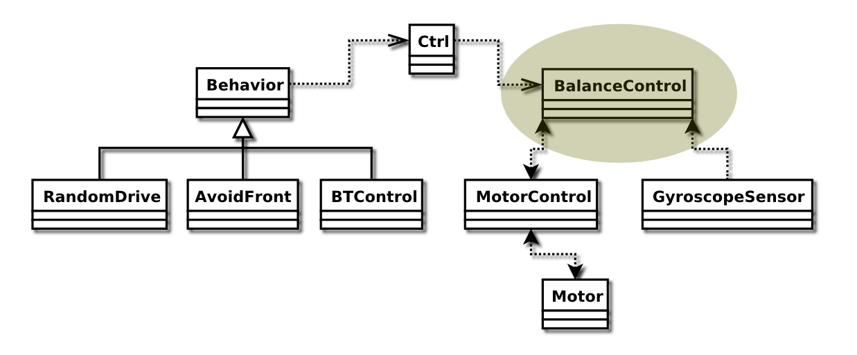 This class contains all the PID magic happening that makes Marvin keep its balance.
The balancing module reads the angles and the angle velocities from the gyroscope and motors, and uses these values (weighted) to feed to the PID control calculation which again produces the new power to apply to the motors.
These are the constants used as weights in PID control, and the error calculation:
| Symbol | Variable | Value |
|---|---|---|
| <latex>$K_p$</latex><texit>$K_p$</texit> | Kp | 1.0 |
| <latex>$K_i$</latex><texit>$K_i$</texit> | Ki | 0.2 |
| <latex>$K_d$</latex><texit>$K_d$</texit> | Kd | 0.2 |
| <latex>$K_\Psi$</latex><texit>$K_\Psi$</texit> | K_psi | 31.9978 |
| <latex>$K_\Phi$</latex><texit>$K_\Phi$</texit> | K_phi | 0.8703 |
| <latex>$K_\dot{\Psi}$</latex><texit>$K_{\dot{\Psi}}$</texit> | K_psidot | 0.6 |
| <latex>$K_\dot{\Phi}$</latex><texit>$K_{\dot{\Phi}}$</texit> | K_phidot | 0.02 |
<latex>$K_p$</latex><texit>$K_p$</texit>, <latex>$K_i$</latex><texit>$K_i$</texit> and <latex>$K_d$</latex><texit>$K_d$</texit> are the weights of the proportional, differential and
integral parts of the PID control. We name the gyroscope angle <latex>$\Psi$</latex><texit>$\Psi$</texit>,
and the Motor angle <latex>$\Phi$</latex><texit>$\Phi$</texit>, and their respective differentiates (angle
velocities) <latex>$\dot{\Psi}$</latex><texit>$\dot{\Psi}$</texit> and <latex>$\dot{\Phi}$</latex><texit>$\dot{\Phi}$</texit>, thus making <latex>$K_\Psi$</latex><texit>$K_\Psi$</texit> the weight of the <latex>$\Psi$</latex><texit>$\Psi$</texit> value in the error calculation, <latex>$K_\dot{\Psi}$</latex><texit>$K_{\dot{\Psi}}$</texit> then weight for the <latex>$\dot{\Psi}$</latex><texit>$\dot{\Psi}$</texit> and so on…
The sleep call at the end of the loop, reflects the max sample speed of the gyroscope, which should be is 300 times per second, 3.33msec between calls, but since the code itself takes up some time, the actual sleep value of 3msec seem to work appropriately.
The controls are added, in two places:
- To make Marvin move forward and backwards we add the tilt offset to the gyroscope angle (at the
gyro.getAngle()call).
- To make Marvin rotate wee add the left and right motor offsets directly to the right and left motor power (at the
motors.setPower(…)call).
The following is an excerpt from the BalanceControl class, showing the inner loop (which is running as a thread), that makes the error calculation, runs it through the PID, and finally adjusts the motor power accordingly.
public class BalanceControl extends Thread
{
  .
  .
  .

  public void run()

  {
    MotorControl motors = new MotorControl(Motor.C, Motor.B);
    GyroscopeSensor gyro = new GyroscopeSensor(SensorPort.S4);

    double int_error = 0.0;
    double prev_error = 0.0;

    while(true) {
      double Psi = gyro.getAngle() + ctrl.tiltAngle();
      double PsiDot = gyro.getAngleVelocity();

      double Phi = motors.getAngle();

      double PhiDot = motors.getAngleVelocity();

      double error = Psi * K_psi + Phi * K_phi + PsiDot * K_psidot + PhiDot * K_phidot;

      int_error += error; // Integral Error

      double deriv_error = error - prev_error; // Derivative Error
      prev_error = error;

      double pw = error * Kp + deriv_error * Kd + int_error * Ki;

      motors.setPower(pw + ctrl.leftMotorOffset(), pw + ctrl.rightMotorOffset());

      try { sleep(3); } catch(java.lang.InterruptedException e) { }
    }
  }
}
The full source code for this class can be found in the file BalanceControl.java in the Marvin code tarball 32)
Hardware Related Issues
At first we experienced severe stability problems as Marvin was highly sensitive to the offset of the gyroscope. The offset calibration did not appear to be stationary and this lead to diverging oscillations, which caused Marvin to crash over and over. (Fortunately the NXT module is quite solid.) We used great effort to find a solution to this problem and though the gyroscope tends to drift over time, we were able to find a stable combination of the tuning parameters causing Marvin to balance for several minutes - using only the tilt angle from the gyroscope and the PID control loop. At this point Marvin was balancing so we tried some preliminary attempts in order for Marvin to move forward/backward. This task was not as easy as expected and therefore the next lab report is devoted to the driving. It is important to notice, that at this point we did not use all the aforementioned states, since all four states contributed to an increasing set of gain combinations - it is not that easy to set all seven gains intuitively! We were only using the integration part of the gyroscope readings, but our suspicion at this point was closing in on the (lack of) states in the control loop. As we finally decided to work with all four states in the control loop, we found a strong combination of the four feedback gains. By adding these extra features we overcame the offset problems of the gyroscope to a satisfying degree. After some longer fine tuning of the parameters, Marvin showed a pretty stable behaviour and hereafter we were confident that he would be able to drive properly. It had to be a matter of finding the right approach, but this problem is addressed in the following lab report. The different attempts to resolve the gyroscope drifting is also adressed in the following lab report.
Lab report 3 - Driving
Date: January 14nd 2009
Duration of activity: 8-16
Participants: Kasper, Bent and Johnny
Project Goal
Make robot able to drive a predefined pattern.
Plan
- Create a Motor Control class that can append extra power to the motors individually to control how the robot is behaving.
Theory
DC Motor Drives
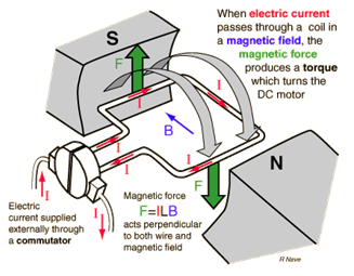
 The Lego Mindstorm kit comes with a set of DC Motors and therefore we shall give a short introduction to the DC motor and the DC motor controller. This will hopefully add nicely to the presentation of the H-bridge and DC servo motors33) given in week 4 of the course. Let us begin with the DC motor.34)
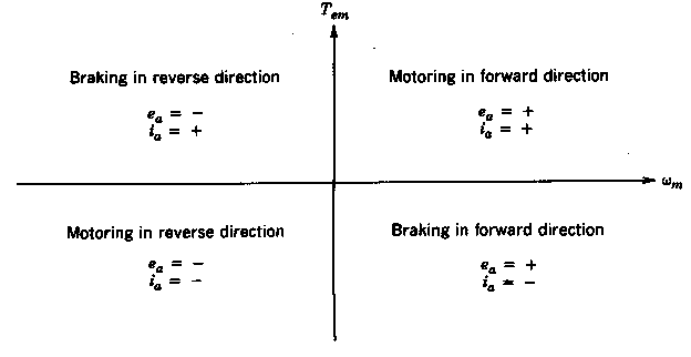
The DC motor is illustrated with a permanent magnet, but in many cases a electromagnet is used instead as it improves the performance of the DC servo motor. In a DC motor the rotor carries the electrical power as opposed to the AC motor, where the stator handles the power. The armature winding needs to be in the rotor of a DC motor to provide a rectification of the voltages and currents, which enables the motor to drive in all four quadrants. As we see on the illustration, the current is supplied externally through a commutator that rotates with the shaft and therefore carbon brushes are used to make contact between the commutator segments and supply terminals. The electric current is supplied through the brushed to the commutator where it passes through a magnetic field via the armature wire, hence the magnetic force produces a motor torque that turns the rotor. This is standard physics, but one very important detail about the physics of the DC motor is the energy of the system. When the motor is running, the system contains energy that originates from the inertia of the motor load, and therefore the motor supply must be able to handle this energy when the motor is stopped or when we request a change of direction. When the motor is breaking the kinetic energy from the motor load inertia is converted into electrical energy. This means that the motor will try to uphold the voltage - meaning that the DC motor is now working as a generator supplying our motor controller, but notice that the direction of the electrical current has changed. In order to operate the DC motor, the controller must therefore be able to handle four-quadrant operation.
Power Electronic Converter
We see that the four quadrants refers to the four combinations of voltage and current directions. As mentioned the motor is actually transferring energy back to the supply when breaking and this requires special attention when designing a motor controller. In order to control the DC motor a Power Electric Converter (PEC) that satisfies the following conditions is needed. 35)
- The converter must allow both output voltage and current to reverse in order to yield a four-quadrant operation.
- For accurate control of position, the average voltage output of the converter should vary linearly with its control input, independent of the load on the motor.
- The converter output should respond as quickly as possible to its control input, thus allowing the converter to be represented essentially by a constant gain without dead time in the overall servo drive system.
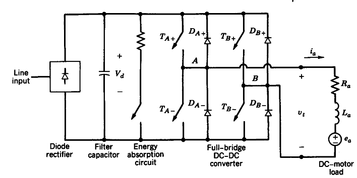
Further demands may be required, but these are essentials and adequate for our purpose. A linear power amplifier would be highly ineffective and therefore a switch mode dc-dc converter is used. A full bridge (H-bridge) converter is in fact capable of operating in all four quadrants and is illustrated on the following diagram.
Observe that it contains an energy absorption circuit in order to waste the kinetic energy from the motor load inertia by heating up a resistor. A more advanced solution would be to store the energy back to the battery, which we may assume in the NXT kit. Lastly we will demonstrate the four-quadrant behaviour of the full-bridge dc-dc converter.
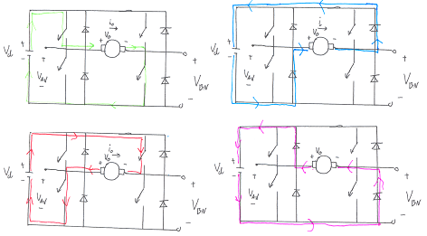
The top left illustration show forward motion, where two transistors are connected to guide the current forward through the DC motor - notice that the transistors are always connected pairwise. As we decide to change direction the transistors are disconnected in the blanking time, whereafter the other two transistors are connected. The rectifiers are mounted anti parallel and works as a valve for the aforementioned extra energy, that is either eliminated by the resister or fed back to the battery. This is illustrated on the top right, which indicates the forward breaking of the motor. Notice how the voltage and current directions are maintained in the breaking phase, since the motor is incapable of altering its direction instantaneous cf. our explanation regarding kinetic energy. The lower left illustrates the backward motion of the motor and finally lower right shows the backward breaking loop. We therefore see that the H-bridge is in fact capable of four quadrant motion, which is cleverly implemented using transistors and rectifiers. (The diagram is simplified, naturally). Fortunately the motor control is linear, which is a requirement in our control loop as it is a linear controller. However, the average voltage output does not vary linear with the control input voltage during the blanking time, which occurs when the motor direction changes. In our case this happens all the time to keep the robot in state of equilibrium and we may therefore expect some non linear behaviour from the motors.
Motor Encoder/Tacho Counter
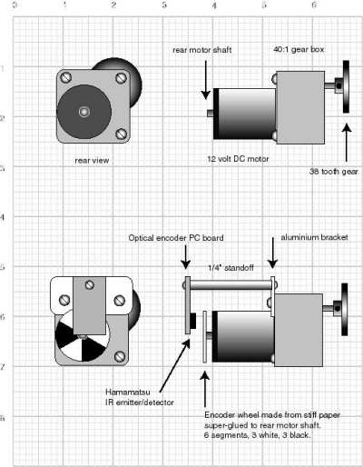
When designing the motors, wheels and drive train, it will almost always be important to have some sort of encoder feedback. In the LeJOS framework there are methods to get readings from the tacho counters and these sensor readings have proven to be very useful when designing a balancing robot cf. the research literature in the introduction. In order to illustrate the concept of an encoder we use this simple set-up, which is explained in the excellent SRS Encoder article by David Anderson36). Imagine a DC motor without an encoder which is illustrated in the top of the figure. If we mount a circular image with a pattern determining our resolution, we can use a simple IR transceiver to get readings back to our micro controller or signal processing unit. In the LEGO Mindstorm Kit37) each motor has a built-in Rotation Sensor. This allows us to control the robot’s movements quite accurate. The Rotation Sensor measures motor rotations in degrees or full rotations [accuracy of +/- one degree]. One rotation is equal to 360 degrees, so if we set a motor to turn 180 degrees, its output shaft will make half a turn. This allows us to evaluate both the body angle and angle velocity of the balancing robot by means of simple differentiation, which is explained in one of the following sections.
Implementation
Right/Left Steering
Now that the robot is balancing it ought to be simple to make it drive around. We expect the controller to maintain its balance even though we apply the necessary offset to the PWM in order to make it move. At first we added a small offset to one wheel and subtracted from the other, which caused the robot to drive in a circle. The robot actually seemed to be more robust when turning and we were able to reach a high speeds when pivoting “on the spot”. Maybe this has to do with the angular momentum that is being build up when turning on the spot - similar to the ice skater doing a pirouette. Also we reduce the slip in the motor by keeping the robot rotating. This can be seen on the following video
As you may have noticed on the video we did also change the tires. The tires in the original model had a course pattern and this caused it to get stuck on the carpet and so the robot did not behave equally on both carpets and hard surfaces. By changing to a very flat and smooth tire we experienced more similar behaviours on different surfaces and this made the tuning of the parameters in the control loop a bit easier.
Forward/Backward Motion
The idea was then to make the robot move forward by adding a small offset on both wheels, but clearly this was not the right approach. Either the controller does not allow the robot to move, or it oscillates and crashes. The reason for this is actually quite clear if we recall our control loop.
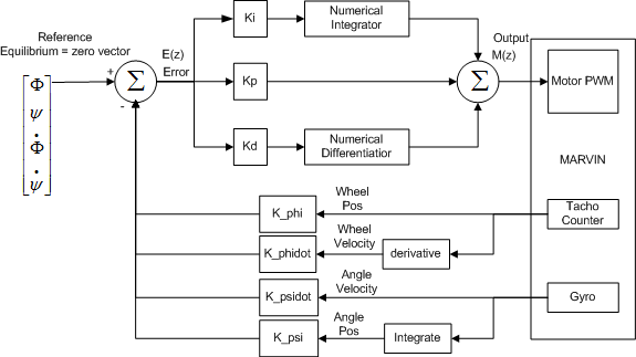
If we apply an offset to both wheels we are removing control from the controller and disturbing the calculated error. Either the control loop will overcome this disturbance by some minor oscillations or it will become unstable as we are really adding to the overshoot. This does not happen when we add a small offset to one wheel and subtract from the other since this does not affect the overall error signal. The natural place to control a closed loop control is of course the reference values, which are applied for each state. The reason that we did not use this approach immediately is probably that the reference values have been left unused as we want all the states to be zero in order for the robot to remain in equilibrium. If a small offset is added to the tilt angle (<latex>\Psi</latex><texit>$\Psi$</texit>) the robot must remain in motion to stay balanced. Although the robot is capable of moving forward and backward it showed an undesired tendency to oscillate between forward and backward commands. As the contra steering used to turn the robot did seem to stabilize the robot, it seemed important to make the robot occupied in between commands by adding a small amount of contra steering. This will keep the motors busy and reduce the slip when the motors are changing from forward to backward motion simultaneously. We used a sine function to add a small offset to one wheel and subtract from the other as the sine function overall should make the robot remain in the same position. The real benefit from this can be found in the high amount of slip in the motors in the instant where they are not active. Without the sine offset, the slip would point in the same direction, but with the small contra steering it actually points in separate directions, hence stabilizing the robot.
Using this approach we are now able to control the robot as expected, thus we are able to make the robot drive a predefined pattern. It is important to mention that the robot still has a tendency to oscillate, which often requires the control loop to “interrupt” the desired motion causing the robot to move unexpected. Therefore the the robot is not able to drive according to the navigation class, but it is satisfactory in order to implement a behaviour control model.
The goal of this lab session was to make Marvin capable of driving a predefined pattern, but we did not specify anything about the accuracy of its position or which type of pattern. We are currently satisfied with the progress and we find the result satisfactory with respect to the next lab session in which we shall implement the behaviour based control model.
Gyroscope Offset Drift Problem
Easy as it seems, we did not arrive at the goal without bumps. We had a very annoying problem, where the gyroscope offset was drifting whenever the robot was not standing still in equilibrium (i.e. driving somewhere).
The offset seemed to drift in the direction of the angle (and thereby driving direction), and the larger the angle, the faster the drifting.
We tried several solutions to the problem, in the following they will be outlined, together with the reasons for why they did not work (apart from the last one which in fact worked):
- The first approach was based on the fact that when the robot was in perfect balance (the angle velocities were below a threshold for some amount of time) we could redefine the angle as zero, thus reset the gyroscope angle. This however would make the robot reset its angle at a position not vertical whenever driving forward, for some period of time long enough to exceed the threshold buffer length.
- Second we used the fact that when the angle offset had reached a certain level, the robot continuously tried to straighten up, resulting in the wheels spinning up to maximum speed in the opposite direction. Based on this observation, we tried to detect when the wheels were driving above a threshold, and thereafter adjust the offset angle towards the actual zero. This did not seem to fix the problem at all, since the time we used to detect the large offset, was way too long for us to prevent Marvin from falling.
- Next we tried to calculate the drift size by multiplying the angle with a constant. We put a lot of effort into tuning this constant, but all in vein. If the drift size can be calculated as a function of the angle, it is certainly not a linear one.
- We had read, on an NXT/gyroscope forum, that there might be a problem with the ADC based on its reference voltage, due to drop in battery level. This lead to an attempt to calculate the drift size based on the current battery level measured against the initial battery level. This however did not seem to be the way to things either, since there were no obvious connection between the battery level and the angle drift.
- We later tried to simply add a constant to the calculated angle after each iteration, and tried to adjust it manually, by modifying it, tweaking it, until we thought it as accurate as we could possibly make it. This seemed to work to a certain point. The drift grew smaller, but never seemed to disappear entirely.
- For some time we suspected the gyroscope reading in itself of being too inaccurate, which lead to a fix, where we replaced every reading with the average of a number of readouts, each with a 3ms interval. This seemed to work while the robot was in balance, but had negative effect when it was tilting fast, since this very same method would dampen the large values of the gyroscope, so this was obviously not a satisfying solution either.
- The last attempt was to simply make a running weighted average of all the gyroscope readings, with an initial value measured by hand. This method was based on the assumption, that the robot would be tilting equally much forward and backwards, which seems plausible. This seemed to work, so that was the solution we chose.
All of these considerations lead to the programming of the MotorControl class.
The MotorControl Class
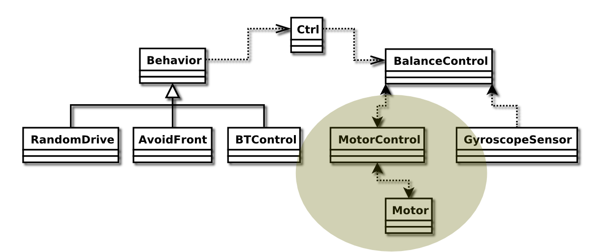 The MotorControl class handles the motors exclusively. It works as a control interface on top of the actual Motor ports, and can report angle and angle velocity (using the TACHO counter) of both of them, as well as set the power and direction.
The small stabilizing algorithm is located at the top of the setPower(…) method. Recall that it makes sure that the gears of the motors are always tightened, to minimize the slack on direction change.
The small amount of power added by the sine function, makes the robot wriggle a little when standing absolutely still, which is actually noticeable when observed carefully.
The motor angle and angle velocity methods simply uses the average of the values from the actual motor ports.
The code for these methods can be seen below:
class MotorControl
{
  private Motor leftMotor;
  private Motor rightMotor;

  .
  .
  .

  public void setPower(double leftPower, double rightPower)
  {
    sin_x += sin_speed;
    int pwl = (int)( leftPower + Math.sin(sin_x) * sin_amp );
    int pwr = (int)( rightPower - Math.sin(sin_x) * sin_amp );

    leftMotor.setSpeed(pwl);
    if(pwl < 0) {
      leftMotor.backward();
    } else if(pwl > 0) {
      leftMotor.forward();
    } else {
      leftMotor.stop();
    }

    rightMotor.setSpeed(pwr);
    if(pwr < 0) {
      rightMotor.backward();
    } else if(pwr > 0) {
      rightMotor.forward();
    } else {
      rightMotor.stop();
    }
  }

  public double getAngle()
  {
    return ((double)leftMotor.getTachoCount() + (double)rightMotor.getTachoCount()) / 2.0;
  }

  public double getAngleVelocity()
  {
    return ((double)leftMotor.getActualSpeed() + (double)rightMotor.getActualSpeed()) / 2.0;
  }
}
Ctrl
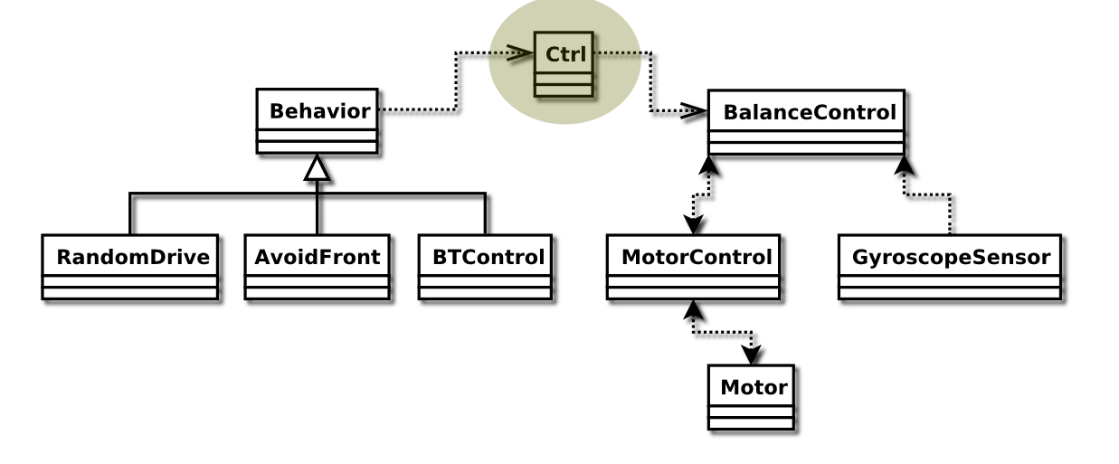 The Ctrl class is used to handle the control parameters of Marvin.
It is used for cross thread communication, and simply sets and reads a number of parameters through synchronized methods.
The parameters are left and right motor power offsets, and gyroscope tilt angle offset.
The way we made Marvin drive in a hard coded path was to set these values directly in the Ctrl class, and use a counter to switch values after a predefined number of iterations (simply increment the counter upon each read call and switch when the value is high enough).
The code for the offsetLeft value can be seen below, the code for rightOffset and tiltOffset works similar.
class Ctrl {
  private double offsetLeft = 0.0;

  .
  .
  .

  public synchronized void setLeftMotorOffset(double offset)
  {
    this.offsetLeft = offset;
  }

  .
  .
  .

  public synchronized double leftMotorOffset()
  {
    return this.offsetLeft;
  }

  .
  .
  .
}
The full source code for these classes can be found in the files MotorControl.java and Ctrl.java in the Marvin code tarball 38)
Lab report 4 - Behaviour Control
Date: January 16nd 2009
Duration of activity: 8-16
Participants: Kasper, Bent and Johnny
Project Goal
Make the robot drive autonomously, avoiding obstacles by means of a behaviour model.
Plan
- Move balance related code to a thread.
- Make control parameters writeable from outside the motor thread to make it possible to drive around.
- Copy code from previous Behaviour project 39).
- Modify the code to make it fit Marvin.
Theory
The Ultrasonic Sensor
Ultrasonic sensors work on a principle similar to radar or sonar by emitting an impulse and interpreting the echoes from radio or sound waves respectively. Ultrasonic sensors generate high frequency sound waves and evaluate the echo which is received back by the sensor. The time interval between the emitted and received signal is then calculated in order to determine a distance to a given object. The ultrasonic sensors are also known as transducers when they both send and receive signals. The Ultrasonic Sensor40) measures distance in centimetres and in inches. It is able to measure distances from 0 to 255 centimetres with a precision of +/- 3 cm. Large sized objects with hard surfaces return the best readings. Objects made of soft fabric or that are curved (like a ball) or are very thin or small can be difficult for the sensor to detect. Note that two or more Ultrasonic Sensors operating in the same room may interrupt each other’s readings.
Knowledge Learned from Previous Lessons
Prior to using a sensor for a specific purpose it is important to investigate the main use for the sensor. For example in lab session 4 41) we used the light-sensor as an input for measuring tilt of the robot. Or in other words, it was not the primary use for the sensor we used it for. Another example is the ultrasonic sensor 42) which operates fairly precise when operated at an angle of 90 degrees to the wall, because is uses echo for measurement. When the angle was shifted to one side the sensor became increasingly inaccurate. Again you have to closely investigate the capabilities and limitations of the sensor one plans to use. As the ultrasonic sensor depends on sound, the primary limitations are echo delays and angle shifts. Therefore the best readings will be available when the sensor is positioned directly in in front of a wall. And the best readings will also be available when to sensor is close to the wall due to the fact that echoes will travel in different directions. These limitations will not be a problem in our project due to the fact that we only use the ultrasonic sensor to avoid that Marvin will hit any walls.
Implementation
The Behavior Class
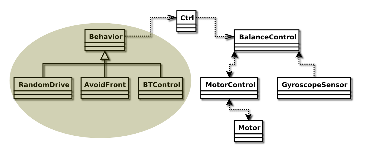 A platform for a behaviour based system with a simple suppression mechanism. An actual behaviour is defined by extending the
 Behavior class. Each behaviour is a single thread of control.
It has access to control the Marvin by means of the control methods (forward, backward, left and right).
However, access can be suppressed so that the motor commands will not be performed while the behaviour is suppressed.
| Variable | Value |
|---|---|
| turnPower | 200 |
| tiltPower | 0.06 |
public class Behavior extends Thread
{
  private ArrayList behaviors;;
  private boolean suppressed;
  private Ctrl ctrl;

  public Behavior(ArrayList behaviors, Ctrl ctrl)
  {
    this.ctrl = ctrl;
    suppressed = false;

    this.setDaemon(true);

    // Clone the Behavior list.
    this.behaviors = new ArrayList();

    for(int i = 0; i < behaviors.size(); i++) {
      Behavior b = (Behavior)behaviors.get(i);
      this.behaviors.add(b);
    }
  }

  public void suppressLower()
  {
    for(int i = 0; i < behaviors.size(); i++) {
      Behavior b = (Behavior)behaviors.get(i);
      b.setSuppress(true);
    }
  }

  .
  .
  .

  public synchronized boolean isSuppressed()
  {
    return suppressed;
  }

  public synchronized void setSuppress(boolean suppress)
  {
    suppressed = suppress;
  }

  public void forward(int period)
  {
    if(!isSuppressed()) {
      ctrl.setLeftMotorOffset(0);
      ctrl.setRightMotorOffset(0);

      for(int time = 0; time < period; time += 10) {
        try { Thread.sleep(10); } catch(InterruptedException e) { }
        ctrl.setTiltAngle(-tiltPower);
      }
    }
  }

  public void right(int period)
  {
    if(!isSuppressed()) {
      ctrl.setLeftMotorOffset(turnPower);
      ctrl.setRightMotorOffset(-turnPower);
      delay(period);
    }
  }

  .
  .
  .

}
The Behavior class has the following 3 subclasses:
The RandomDrive Class
This behaviour drives in one of four random directions for a random number of milliseconds. All of these numbers are computed using a random function from Java Math library.
The AvoidFront Class
Implemented using a ultrasonic sensor. The behaviour activates a backward motion and do this for a number of milliseconds to back away from the obstacle. Afterwards Marvin stops and turns right corresponding to an approximately 90 degree turn. The code for the essential parts of the AvoidFront class can be seen below as an illustrative example of how behaviours are implemented in general.
public class AvoidFront extends Behavior
{
  .
  .
  .

  public void run()
  {
    UltrasonicSensor us = new UltrasonicSensor(SensorPort.S2);
    int tooCloseThreshold = 20; // cm

    while (true) {
      int distance = us.getDistance();
      while(distance > tooCloseThreshold) {
        distance = us.getDistance();
        delay(100);
      }

      suppressLower();

      backward(5000);
      right(1200);
      stop(2000);

      unsuppressLower();
    }
  }
}
The BTController Class
The thread handles bluetooth communication in order to control Marvin with a remote control. The arrow keys on the computer is used instead of a remote. This class will be covered in detail in the next lab report.
The full source code for these classes can be found in the files Behavior.java, RandomDrive.java, BTController.java and AvoidWall.java in the Marvin code tarball 43)
Lab report 5 - Bluetooth controlled robot
Date: January 19nd 2009
Duration of activity: 8-16
Participants: Kasper, Bent and Johnny
Project Goal
Make robot remote controlled from the PC through bluetooth.
Plan
- Make a bluetooth client code Behaviour on the Marvin, that can receive numbers and act on them.
- Make PC bluetooth application read from keyboard arrows to determine control direction.
Theory
The Protocol
From wikipedia: “Bluetooth is a wireless protocol for exchanging data over short distances”44). The NXT hosts a bluetooth communication device, and is capable of communicating at up to approximately 10 metres distance.
LeJOS has built an entire framework for bluetooth communication, over normal Java input/output streams.
45)
We do not want to go further into the details of the protocol itself, but the way the device is shared can eventually end up in data loss46). We however do not care about this, since we intend to use it to send loads of control keycodes to the robot without worrying whether they will all arrive safely at the destination.
On the PC LeJOS has also made a bluetooth interface. This works exactly the same as the one on the NXT, and we therefore simply had to make a connection (listening on the NXT and connecting on the PC) and then creating input/output streams, to make the communication work as intended.
LeJOS has put a lot of effort into making the bluetooth communication easy to use, and the implementation were therefore quite straight forward. Observe the resulting code below.
We experienced a lot of slowdown in the balancing thread whenever the bluetooth communication was running, and we had to disable it entirely at numerous occasions to avoid the robot falling over.
We later discovered that the problem could be worked around by disabling some of the other behaviour threads to release more resources, and make Marvin rebalance itself while driving around remote controlled.
Here is a movie of the resulting remote controlled robot, with all other behaviours disabled:
 CBRJdHbWyV4
As it can be seen from the video, Marvin is not exactly reacting real-time to the control changes. This is due to the way the BTControl has been implemented, but also because the tilt reference must be incremented gradually, but still has to reach a certain level before an actual forward or backward motion can be seen. Making this incrementation more rapid (and thereby making the reaction faster) will cause Marvin to nosedive.
Implementation
The BTControl Class
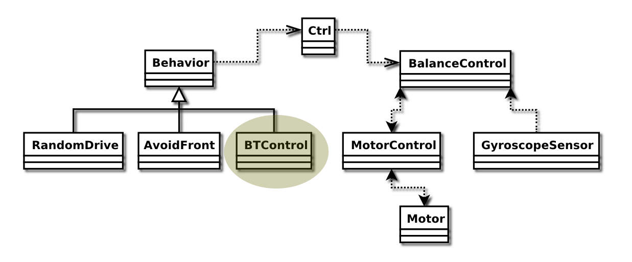 Bluetooth control behaviour. It reads integers from a bluetooth input stream, interpreting them as keycodes.
It reacts only on the keycodes connected with the arrow keys (up, down, left, right) and tells Marvin to drive accordingly.
| Key | KeyCode | Variable |
|---|---|---|
| left | 37 | directionLeft |
| right | 39 | directionRight |
| up | 38 | directionForward |
| down | 40 | directionBackward |
All exception handlers have been removed to improve on readability:
public class BTController extends Behavior
{
  .
  .
  .

  public void run()
  {
    NXTConnection conn = Bluetooth.waitForConnection();
    DataInputStream istream = conn.openDataInputStream();

    while(true) {
      if(istream.available() > 0) direction = istream.readInt();
      else delay(200);

      if(direction >= directionLeft && direction <= directionBackward) {
        suppressLower();
        switch(direction) {
        case directionLeft:
          left(200);


          break;

        case directionRight:
          right(200);
          break;

        case directionForward:
          forward(200);
          break;

        case directionBackward:
          backward(200);
          break;
        }
        unsuppressLower();

        // Empty input buffer... we only want to use the latest keystroke.
        while(istream.available() > 1) istream.readInt();
      }
    }
  }
}
The PCController Class
On the PC, we use a window (JFrame) to capture keyboard input and redirect their keycode values to the bluetooth stream.
NXTComm nxtComm = NXTCommFactory.createNXTComm(NXTCommFactory.BLUETOOTH);
NXTInfo nxtInfo = new NXTInfo("Marvin", "00:16:53:06:E3:36");
nxtComm.open(nxtInfo);

OutputStream os = nxtComm.getOutputStream();
final DataOutputStream dos = new DataOutputStream(os);

JFrame frame = ...

frame.addKeyListener(new KeyListener() {
  public void keyPressed(KeyEvent e) {
    dos.writeInt(e.getKeyCode());
    dos.flush();
  }
  public void keyReleased(KeyEvent e) {}
  public void keyTyped(KeyEvent e) {}
});
The full source code for both of these classes can be found in the files BTController.java and PCController.java in the Marvin code tarball 47). See the marvinController script file in the same tarball, to get an idea of how to run the bluetooth client program.
Improvements
Even though we are quite pleased with the performance of Marvin, there are some issues that we would like to improve in the future if the opportunity presents itself.
Marvin is able to balance and drive around randomly while avoiding obstacles. He is also able to be remotely controlled via Bluetooth. However these two behaviours do not operate well together due to resource sharing problems in the threads. We did not find a solution to this problem, but keeping them both at the same time had a high priority in the group, since it is an essential part of the behaviour architecture. The problem might be solved by changing to another framework with a different thread implementation, but we have not investigated this further.
We chose to use a PID controller because it had been introduced during the course, but it could be interesting to investigate some other controllers and evaluate their performance as well. The controllers of interest could be an LQR controller or/and a Pole-Placement Controller. These are mere a few amongst many. We are curios as to whether it could be possible to further optimize the PID control parameters for better balancing and robustness, or if it has been pushed to its limits whereas we would have to turn to other controller algorithms to achieve better results.
In order to further optimize the PID control parameters (or any other parameters of interest), it would be nice to have an online tuning method through a PC GUI application, communicating with the robot by means of bluetooth.
Conclusion
In lab 1148) we outlined the project with its path of progression, problems and goals. To summarize it we wanted to “be able to show a bluetooth remote controlled gyro-balancing robot, driving autonomously when not controlled, capable of avoiding obstacles.”.
During the entirety of the unwinding of the project, we kept the original goals in mind, and tried to keep as close to them as possible. We did not expect, but hoped, to accomplish all of them, however contrary to our expectations, we managed to achieve all, but one (the GUI).
Conclusively we consider this project a success.
